Training and Evaluating CIFAR10 Image Data with TinyVGG Model Architecture Built With PyTorch


Towards the end of my internship, I decided to dive into deep learning and I am super excited to announce that this blog post is about sharing my thought process on the first computer vision project I did.
I worked on the CIFAR10 data set using the TinyVGG Model Architecture using Pytorch. The model evaluation score was 81% which was a huge improvement from the 62% that was scored on the baseline model.
PROJECT GOAL
The goal of this project is to use an improved existing model architecture, In this case, using the TinyVGG model to accurately look at a picture and tell us if the picture is one of the following: airplane, automobile, bird, cat, deer, dog, frog, horse, ship, truck. The dataset used for training the model was the famous CIFAR10 dataset (you can read more about it [here].
Importing Libraries
The following Libraries were needed for the success of this project.
import torchvision # Because we are working with a vision data
from torchvision import datasets, transforms # loading and transforming data
import matplotlib.pyplot as plt # For Visualization
import torch # needed some packages that are embedded in this library
from torch import nn # for creating models
import numpy as np # for all the math stuffs
from torch.utils.data.dataloader import DataLoader # For turning data into batches
from torchmetrics import Accuracy # Evaluation metric
from tqdm.auto import tqdm # fancy visual
from torchvision.transforms import AutoAugment, AutoAugmentPolicy # for augmenting data
# Creating device agnostic code in order to ensure that that the codes can run on both GPU and cpu
device= 'cuda' if torch.cuda.is_available() else 'cpu'
Data loading and Augmentation
Before I start writing codes, I want to emphasize that I have trained an unaugmented version of this data on the model to get the baseline score which is 71% after which I worked on improving the data and this article is about the improved version of the project.
Now before downloading the data, I performed data augmentation where I used the auto data augmentation policy for CIFAR10 on the trained data, I also transformed both train and test data to tensors as Pytorch only works with tensors and the data was in Numpy arrays, Then I applied random horizontal flip on the train data as the model was not generalizing well on the test data.
# Transform data
train_transform=
transforms.Compose([transforms.AutoAugment(policy=AutoAugmentPolicy.CIFAR10),
                                     transforms.RandomHorizontalFlip(p=0.5),
                                     transforms.ToTensor(),
                                      ])

test_transform= transforms.Compose([transforms.ToTensor()])
The transforms.Compose library was used to map all the transformations together. Noticed how no transformation was performed on the test data? It is because it is the unknown data our model is supposed to test or evaluate to see how well it is generalizing on data it has not been trained on.
# downloading the dataset
train_data= torchvision.datasets.CIFAR10(root= 'cifa_dataset',
                                         train= True,
                                         transform=train_transform,
                                         download= True,
                                         target_transform=None)
test_data= torchvision.datasets.CIFAR10(root= 'cifa_dataset_test',
                                        train= False,
                                        transform=test_transform,
                                        download= True,
                                        target_transform=None)
The data was loaded and explored. It was noted that the data was in 32*32 with three color channels and a visualization function was built to avoid code repetition.
def show_image(image_data, class_names, class_preds = None):
  """
  this functions takes in 9 batches of array of numbers in height, weight and        color format functions
  and returns a 3 by 3 visualization of the data

  args
  ----
  image_data: (array) arrays of numbers in height, weight and color format
  class_names: (list) class names of the data
  class_preds: (Optional) if available, The Target name that the model predicted
  smooth:(Boolean) either pixelated or smooth version of the dataset
  """
  classes_names= train_data.classes
  fig= plt.figure(figsize=(9,9))
  rows, cols=3,3
  for i in range(1, rows*cols+1):
    img= image_data[i]
    label= classes_names[class_names[i]]
    fig.add_subplot(rows, cols, i)
    plt.imshow(img,interpolation_stage='rgba')

    if class_preds is None:
      plt.title(label)
    else:
      pred= classes_names[class_preds[i]]
      title_text= f'Truth:{label} | Pred:{pred}'
      if label==pred:
        plt.title(title_text, fontsize=10, c='g')
      else:
        plt.title(title_text, fontsize=10, c='r')

    plt.axis(False)
# To view the first 9 pictures of the dataset without transformations
  show_image(image_data=train_data.data[: 10], class_names= train_data.targets[: 10])
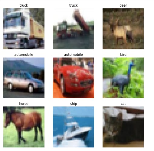
Getting the data ready for training
The untransformed data was visualized in the figure above but the transformed data will be visualized later on. The transformed data was shuffled and divided into batches after which it was visualized.
train_dataloader= DataLoader(dataset= train_data,
                             batch_size= 64,
                             shuffle= True,
                             )
test_dataloader= DataLoader(dataset=test_data,
                            batch_size=64,
                            shuffle=True,
                            )
# Exploring transformed data in batches
train_feature_batch, train_label_batch= next(iter(train_dataloader))
# Changed the shape because matplotlib takes in image data in [Batchsize, height, width, color_channels] format which is different from the shape the tensor has been converted to.
show_image(image_data=train_feature_batch[: 10].permute(0,2,3,1), class_names= train_label_batch[: 10])
Creating a training and test loop function
I created a function for this to avoid code repetition
def training_loop(model, dataloader, accuracy_fn, loss_fn, device, optimizer):
  '''
  args
  -----
  model: torch model architecture
  epochs: [int] number of epochs
  dataloader:[torch.tensor] data in batches
  accuracy_fn: accuracy function
  loss_fn: loss function
  device: either cpu or cuda
  optimizer: optimizer function

  returns accuracy and loss function metrics of the trained data
  '''
  train_loss=0
  train_acc=0
  model.train()
  for batch, (X,y) in enumerate(dataloader):
    X, y= X.to(device), y.to(device)
    y_logits= model(X)
    loss = loss_fn(y_logits, y)
    train_loss += loss.item()
    train_acc += accuracy_fn(y, y_logits.argmax(dim=1)).item()
    optimizer.zero_grad()
    loss.backward()
    optimizer.step()

  train_loss /= len(dataloader)
  train_acc /= len(dataloader)

  return train_loss, train_acc
def test_loop(model: torch.nn.Module,dataloader, accuracy_fn, loss_fn, device):
  '''
  args
  -----
  model: torch model architecture
  epochs: [int] number of epochs
  dataloader:[torch.tensor] data in batches
  accuracy_fn: accuracy function
  loss_fn: loss function
  device: either cpu or cuda

  returns accuracy and loss function metrics of the test data
  '''
  test_loss=0
  test_acc=0
  model.eval()
  with torch.inference_mode():
    for X, y in dataloader:
      X, y= X.to(device), y.to(device)
      y_pred= model(X)
      loss= loss_fn(y_pred, y)
      test_loss += loss.item()
      test_acc += accuracy_fn(y, y_pred.argmax(dim=1)).item()
    test_loss /= len(dataloader)
    test_acc /= len(dataloader)

    return test_loss, test_acc
Creating a function to train the model
def training_function(model, optimizer, train_dataloader, test_dataloader, accuracy_fn, loss_fn, device, epochs):
  '''
  args
  -----
  model: torch model architecture
  epochs: [int] number of epochs
  train_dataloader: trained data in batches
  test_dataloader: test data in batches
  accuracy_fn: accuracy function
  loss_fn: loss function
  device: either cpu or cuda
  optimizer: optimizer function

  returns accuracy and loss function metrics of the trained and test data
  '''

  result= {'train_loss': [],
          'train_Acc': [],
          'test_loss': [],
          'test_Acc':[]}
  for epoch in tqdm(range(epochs)):
    train_loss, train_acc= training_loop(model=model,
                                         dataloader= train_dataloader,
                                         accuracy_fn= accuracy_fn,
                                         loss_fn= loss_fn,
                                         device= device,
                                         optimizer= optimizer)
    test_loss, test_acc= test_loop(model= model, dataloader=test_dataloader, accuracy_fn=accuracy_fn, loss_fn= loss_fn, device=device)

    print (f'Epochs: {epoch} | train loss {train_loss:.4f} | Train acc: {train_acc:.4f} |test_loss {test_loss:.4f}| test acc {test_acc:.4f}')

    result['train_loss'].append(train_loss)
    result['test_loss'].append(test_loss)
    result['train_Acc'].append(train_acc)
    result['test_Acc'].append(test_acc)

  return result
Creating loss function, evaluation metric and optimization function.
For this, any loss function or optimization can be used but I used cross entropy loss because I was working on a multiclass classification problem and the loss function work well with this dataset. The SGD (Stochastic gradient Descent) optimizer was used and the learning rate was set to 0.1. The metric used to score the model was Accuracy.
accuracy= Accuracy(task= 'multiclass', num_classes= 10).to(device)
loss_fn= nn.CrossEntropyLoss()
optimizer_conv= torch.optim.SGD(model_conv.parameters(), lr=0.1)
Creating the model
The model used was replicated from the CNN explainer website but it was slightly improved upon as 1 dimension was added to the pad.
class TinyVGGModel(nn.Module):
  '''
  Model architecture that replicates the tinyVGG model from
  CNN explainer website.
  '''
  def __init__(self, input_shape: int, hidden_shape: int, output_shape:int):
    super().__init__()
    self.conv_block= nn.Sequential(
        nn.Conv2d(in_channels= input_shape,# in_channels = no of channels in visual data. it is usually input shape
                  out_channels= hidden_shape,
                  kernel_size= 3,
                  stride=1,
                  padding=1),

        nn.ReLU(),
        nn.Conv2d(in_channels= hidden_shape,
                  out_channels=hidden_shape,
                  kernel_size=3,
                  stride=1,
                  padding=1),
        nn.ReLU(),
        nn.MaxPool2d(kernel_size=2)
        )

    self.conv_block_2= nn.Sequential(
        nn.Conv2d(in_channels= hidden_shape,
                  out_channels=hidden_shape,
                  kernel_size=3,
                  stride=1,
                  padding=1),
        nn.ReLU(),
        nn.Conv2d(in_channels= hidden_shape,
                  out_channels= hidden_shape,
                  kernel_size= 3,
                  padding=1,
                  stride=1),
        nn.ReLU(),
        nn.MaxPool2d(kernel_size=2)
        )

  # the hidden shape was muliplied by 64 because the shape that is coming out of the conv2 layer has been flattened
    self.classifier_layer= nn.Sequential(
        nn.Flatten(),
        nn.Linear(in_features= hidden_shape*8*8, out_features= hidden_shape),
        nn.ReLU(),
        nn.Linear(in_features=hidden_shape, out_features= output_shape)
    )

  def forward(self, x):
    x= self.conv_block(x)
    x= self.conv_block_2(x)
    x= self.classifier_layer(x)
    return x
Instantiating the model and sending it to the target device (in this case, any available device)
torch.manual_seed(42)
# input data have only one color chanel
model_conv= TinyVGGModel(input_shape=3,
                               hidden_shape=250,
                               output_shape=len(class_names)).to(device)
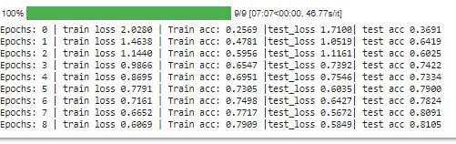
Training the data using the model_conv
model_conv_result= training_function(model=model_conv,
                  epochs=9,
                  train_dataloader= train_dataloader,
                  test_dataloader= test_dataloader,
                  accuracy_fn= accuracy,
                  loss_fn= loss_fn,
                  device= device,
                  optimizer= optimizer_conv)
The model loop through the data 9 times and the following score was gotten from each epoch
Creating evaluation function and evaluating the model
def eval_model(model, dataloader, accuracy_fn, loss_fn, device):
  test_loss= 0
  test_acc=0
  model.eval()
  with torch.inference_mode():
    for X, y in dataloader:
      X,y= X.to(device), y.to(device)
      y_pred= model(X)
      test_loss += loss_fn(y_pred, y)
      test_acc += accuracy_fn(y, y_pred.argmax(dim=1))
    test_loss /= len(dataloader)
    test_acc /= len(dataloader)

    return {
        'model name': model.__class__.__name__,
        'accuracy': test_acc.item(),
        'loss': test_loss.item()
    }
# Evaluating the model
eval_model(model= model_conv, dataloader= test_dataloader, accuracy_fn= accuracy, loss_fn= loss_fn, device= device )
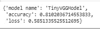
The model was evaluated and it scored 81% on the test data (yay).
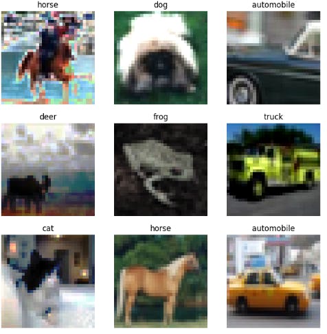
Making predictions with our model
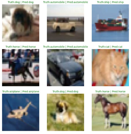
The model was used to make predictions on the data and it was with the 'show_image function' visualized to show how it is performing against the real target value
### Make predictions
pred_list= []
model_conv.to(device)
model_conv.eval()
with torch.inference_mode():
  for X, y in test_data:
    X= X.to(device)
    X= torch.unsqueeze(X, dim=0)
    y_pred= model_conv(X)
    y_pred= y_pred.argmax(dim=1)
    pred_list.append(y_pred.cpu())
pred_list= torch.stack(pred_list)

X= test_data.data
y= test_data.targets
# Visualizing the data with our show image function
show_image(image_data= X[199:209], class_names= y[199:209], class_preds= pred_list[199: 209])
Using confusion matrix metric to see how our model is performing on various classes
# the targets will be converted from list to tensors because we are torchmetrics and it work well with tensors
target= torch.tensor(test_data.targets)
# the prediction list was squeezed in order to remove an extra dimension
pred_list= pred_list.squeeze()

from torchmetrics import ConfusionMatrix
from mlxtend.plotting import plot_confusion_matrix

# setup confusion instance and compare predictions to target
confmat= ConfusionMatrix(num_classes= len(class_names), task= 'multiclass')
conf_tensor= confmat(preds= pred_list, target=target)
# create a graphical representation of the confusion matrix and change tensor to numpy array
fig, ax= plot_confusion_matrix(conf_mat=conf_tensor.numpy(), class_names= class_names, figsize= (10,7) )
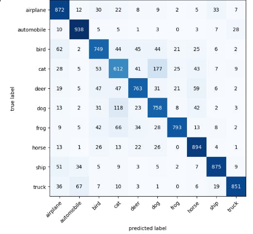
Conclusion
In the confusion matrix, it was discovered that the model wrongly predicted some pictures as others. For example, dogs as cats and cats as dogs. This could be as a result of mislabelling, or the model not having enough data to work with and the metric could get better with using a higher performing model architecture, training the model for longer or generally tweaking the model to see what works. The notebook used for this project can be found here